Page 185 - IJES Special Issues for AIEC2016

International Journal of Environment and Sustainability, 2016, 5(2): 72-88 85

Table 8 and 60 for NOx and O3 while SO2 produced an ex-
orbitantly high value of 327 (Table 10).
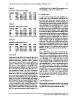
Parameters with priority as NOx
4. Conclusions
Pollutant RMSE r2 MAPE NSE ACFT
NOx 14.834 0.396 23.148 0.341 0.966 A simple method of optimizing the AQMN is pro-
CO 0.565 0.285 73.538 0.275 1.183 posed using GIS, interpolation techniques and
O3 10.736 0.815 85.331 0.432 1.438 historical data. Existing air quality stations are
SO2 37.826 0.109 198.364 -0.194 0.900 systematically eliminated, and the missing data
is filled in using the most appropriate interpola-
Table 9 tion technique. The interpolated data is then
compared with the observed data. Pre-defined
Parameters with priority as SO2 performance measures RMSE, MAPE and r2 were
used to check the accuracy of the interpolated
Pollutant RMSE r2 MAPE NSE ACFT data. NSE and ACFT supported the validity of the
SO2 5.125 0.582 25.128 0.431 1.139 interpolated data. The process was simulated for
O3 11.834 0.550 28.723 0.496 0.929 several sets of observed data using an algorithm
NOx 26.512 0.063 51.687 0.045 1.101 developed in GIS environment. In order to
CO 0.740 0.182 80.081 0.141 1.038 achieve a MAPE value of 25 or less, no combina-
tion of stations could be eliminated for all the
Table 10 pollutants. The pollutants could be prioritized to
achieve the most optimal scenario. The results of
Parameters with priority as CO the prioritization showed that the most optimal
scenario is for the SO2 stations, which achieved
Pollutant RMSE r2 MAPE NSE ACFT MAPE for O3, NOx and CO about 28, 51 and 80, re-
CO 0.236 0.665 25.181 0.647 0.953 spectively.
NOx 17.480 0.287 31.760 0.283 1.047
O3 15.769 0.343 60.332 0.310 1.004 This methodology proves to be useful to the de-
SO2 20.571 0.149 327.356 -1.631 3.067 cision makers to find optimal numbers of sta-
tions that are needed without compromising the
3.5 Overall coverage of the concentrations across the study
area. Although it is a simple procedure, it does
As observed from Tables 2, 3, 4 and 5, there is no have a few limitations. A continuous set of data is
single station that is common among the list of required to get reliable simulation results. Due to
possible elimination stations. Table 6 outlines the unavailability of such a continuous dataset,
the stations required against each pollutant to the staggered dataset is averaged as hourly data
achieve a MAPE level of 25. This indicates that for a day and simulated in the present case study.
the sources of the pollutants are highly varied Secondly, the process is computing intensive, re-
with respect to the location. It will be up to the quiring large computing resources, although
decision maker to prioritize the pollutant and se- such resources are not very expensive these
lect the stations. Tables 7, 8, 9 and 10 illustrate days. Lastly, more parameters can be included in
the statistical parameters taking the priority sta- the performance measures to get the most ap-
tions for O3, NOx, SO2 and CO, respectively. For propriate results.
the case of O3 as priority, MAPE for NOx and CO is
about 57 and 82, while SO2 has a very high MAPE Acknowledgements
value of over 240. Considering NOx as priority,
MAPE value for CO and O3 were about 73 and 85. We gratefully acknowledge the financial support
In this case, SO2 also has a very high MAPE (over of King Abdulaziz City for Science and Technol-
198) as shown in Table 8. The MAPE value of O3 ogy (KACST) under grant number 32-594.
and NOx were less than 50 in the case of SO2 pri-
ority stations, while CO was a little over 80. Tak-
ing CO as priority produced a MAPE value of 31

Science Target Inc. www.sciencetarget.com