Page 178 - IJES Special Issues for AIEC2016

78 © Shareef, Husain, and Alharbi 2016 | Optimal Air Quality Monitoring Network

measures are compared with the pre-defined ArcGIS (ESRI, Redlands) exposes several func-
threshold limits, and if the measures are within tions to run the interpolations and extract the
the limit, they are stored in the possible station necessary data. These functions were custom-
combinations array C(). ized to run the simulation process through Mi-
crosoft Visual Basic for application (VBA) envi-
2.3.7 Step 7: Repeat for another Station Com- ronment in ArcGIS.
bination
3. Results and Discussion
The process is repeated for another station com-
bination until all the combinations are ex- The pollutant concentration data was collected
hausted. from 16 stations as shown in Figure 2. It is as-
sumed that a minimum of eight stations are
2.3.8 Step 8: Finding the Best Possible Station needed to produce reliable interpolated maps.
Combination Therefore, up to eight possible elimination sce-
narios were simulated. Table 1 outlines the sim-
The best possible station combinations can be ulation details such as the number of stations to
chosen from the list of possible station combina- be eliminated, possible number of combinations,
tions array C(). The decision maker can then number of simulations and the approximate time
choose from the list of possible station combina- of simulation (on a high end PC). As seen in the
tions, which can be eliminated from the AQMN. table, the station combinations and the compu-
ting power required increase with the increase
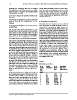
2.4 Study Location and Field Measurements in number of stations. The methodology pro-
posed in this study is tested on the four pollu-
The proposed methodology is applied to the city tants O3, NOx and SO2 and CO, and the results of
of Riyadh, Saudi Arabia. The city is divided into the simulations are discussed as follows. The in-
sixteen cells that are identical in area, and each terpolation was performed using the IDW,
cell is 12 km x 12 km. The measurements were Spline, OK, UK and NN methods. The IDW and UK
carried out intermittently from September 2011 outperformed other methods, particularly in
to September 2012. Most of the measurements terms of producing lower RMSE, MAPE values
have been conducted approximately in the cen- and a higher value of r2.
ter of each cell (Figure 2) with two equipped mo-
bile air quality monitoring stations capable of Table 1
monitoring meteorological variables as well as
CO, O3, NOx, CH4, OC, EC and PM2.5. However, the Simulation parameters
methodology suggested in this study is imple-
mented for the following four criteria pollutants: No. of Possible No. of Approximate
SO2, NOx, O3 and CO. The type of sensors used stations combinations simula- time of sim-
with their respective method of monitoring for to be tions ulation (hours)
the pollutants utilized in this study are NO, NO2 elimi-
and NOx- Chemiluminescence; CO-Dual Beam nated 16 1,920 0.3
NDIR; O3-UV Photometer and SO2- UV Fluores- 1 120 14,400 2.25
cence. 2 560 67,200 10.5
3 1,820 218,400 34
As the measurements are staggered, in order to 4 4,368 524,160 81
get a continuous dataset, 24 datasets were pre- 5 8,008 960,960 150
pared from the available measurements by aver- 6 11,440 1,372,800 214
aging the hourly measurements for the entire 7 12,870 1,544,400 241
study period for all the 16 stations. These 24 da- 8
tasets were used for the simulation to create the
raster with different interpolation techniques
and compared with the observed values. ESRI’s

Science Target Inc. www.sciencetarget.com